Abstract
Adaptive learning systems must repeatedly answer a deceptively simple question: given everything the system knows about a learner right now, what task should be presented next? Current solutions rely on item-response calibration, difficulty estimation, or symptom-matched recommendation rules, each of which captures only a fragment of the determinants of learner engagement and progress. We propose that expected free energy (EFE), the central decision quantity in Active Inference, provides a single computational criterion that unifies these fragments. Specifically, EFE decomposes into three components with direct measurement correlates: precision γ (indexed by heart rate variability), Bayesian information gain I (defined over a learner's skill belief), and pragmatic value U (operationalized as goal–task alignment). The next-task selector minimizes G = −γ·(I + U) over an admissible task library. We formalize the algorithm, specify four sub-modules, and evaluate it in silico on a synthetic cohort of 1,000 learners stratified by developmental level (Fischer levels 7–13) and clinical status. Across four pre-specified hypotheses, the EFE selector (a) predicted engagement from precision (AUC = 0.86), (b) showed an inverted-U learning-rate curve over information gain with optimum at I ≈ 1.0 nats, (c) exhibited a stage-dependent shift from pragmatic to epistemic weighting from Fischer L7 to L13, and (d) outperformed difficulty-only, random, and symptom-only baselines on both engagement and learning-rate criteria. We discuss limitations of synthetic validation, outline a four-phase prospective validation roadmap including an N = 5 case series (initiated May 2026) and N = 200 multi-site cohort, and consider implications for self-regulated learning theory and clinical decision support.
1. Introduction
Among the practical questions that recur across educational technology, intelligent tutoring, neurofeedback training, and clinical psychotherapy, none arises more often than this: given everything we know about this learner right now, what should we ask them to do next? The question is unavoidable because each interaction in a learning sequence presents a fork. Choose a task too easy and the learner disengages from boredom or completes it without measurable change. Choose too hard and the learner abandons it, withdraws, or completes it in a way that consolidates rather than corrects misconception. Choose a task that is well-calibrated to current skill but disconnected from the learner's stated goal and the system trains a capability that the learner will not use. Choose a task that matches the goal but ignores the learner's present physiological state and the system delivers a recommendation that, however well-targeted in principle, will not be enacted (Zimmerman, 2000; Bjork & Bjork, 2011; Porges, 2007).
The empirical literature on adaptive learning has developed sophisticated answers to specialized versions of this question. Item-response theory provides a principled framework for matching item difficulty to learner ability when the goal is psychometric measurement (van der Linden & Glas, 2010). Bayesian knowledge tracing estimates learner mastery of granular skills from interaction histories and supports skill-level adaptation in intelligent tutoring systems (Yudelson et al., 2013; Pelánek, 2017). Multi-armed bandit and contextual bandit algorithms balance exploration and exploitation in recommendation systems and have been applied to educational sequencing (Clement et al., 2015; Bassen et al., 2020). Spaced-repetition algorithms exploit forgetting curves to time review (Settles & Meeder, 2016). Recent work on adaptive instruction with large language models has extended these approaches to open-ended dialogue (Kasneci et al., 2023; Aleven et al., 2023). Each of these literatures has contributed measurable improvements within its scope.
Yet none of these approaches addresses the full set of constraints that govern whether a particular next task is the right one for this learner at this moment. Item-response models do not represent goals. Knowledge tracing models do not represent physiological state. Bandit algorithms do not represent developmental hierarchy. Spaced-repetition algorithms presume that retention is the optimization target, which is true for some learning contexts and false for others (e.g., regulation training, performance optimization, therapeutic skill acquisition). The result, in practice, is that adaptive learning systems are either narrow (optimizing one criterion within one domain) or eclectic (combining heuristics that work most of the time but cannot be derived from any single principle).
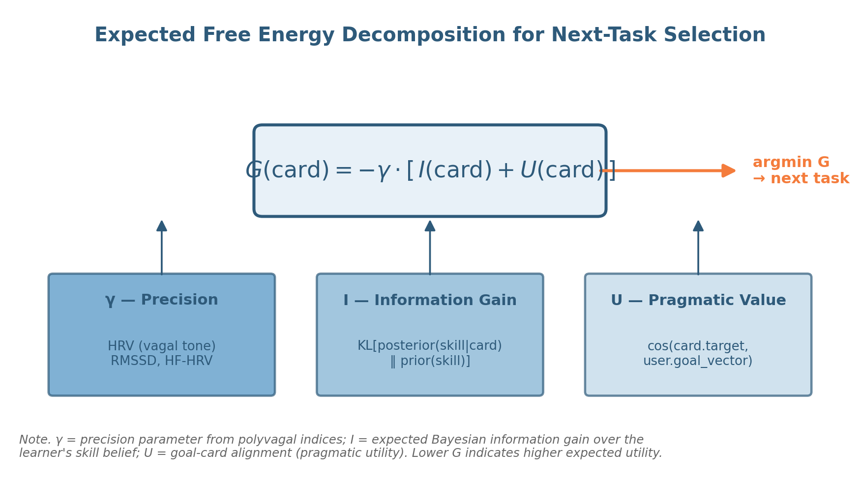
This article proposes that a single computational principle—the minimization of expected free energy (EFE) over candidate actions, central to the Active Inference framework (Friston et al., 2017; Parr et al., 2022)—can serve as the missing unification. Active Inference treats action selection as inference: the agent selects the action whose expected consequences best balance two terms, the expected reduction of uncertainty about the world (epistemic value) and the expected alignment of outcomes with prior preferences (pragmatic value). When this decision is contextualized by a precision parameter γ that gates how strongly preferences and beliefs influence action, the formal structure of EFE becomes a natural fit for next-task selection in self-regulated learning. The learner's skill belief is the inference target. The information gain about that belief from candidate tasks is the epistemic value. The alignment between candidate-task outcomes and the learner's declared goals is the pragmatic value. The precision parameter is the modulator that determines whether the system should select for sharp learning gain (high γ) or for gentle re-engagement (low γ). The criterion is one expression: G = −γ·(I + U), minimized over the candidate library.
1.1 The Specific Problem
We narrow the scope of the present article to a single, specific algorithmic problem: at decision time t, given (a) a vector of physiological and behavioral state inputs S_t for a single learner, (b) a posterior distribution over the learner's skill level on each of five developmentally graded axes, (c) a declared goal vector reflecting the learner's near-term aims, and (d) a finite library of candidate tasks each annotated with a target skill profile and a goal-relevance profile, output a single recommended task to be delivered next. The remaining stages of the system—task delivery, response capture, belief update—are presumed by the algorithm but not the subject of optimization. The optimization target is the selection rule itself.
Framing the problem this narrowly carries three advantages. First, it permits a falsifiable formulation: the proposed selector either improves on appropriate baselines under appropriate evaluation criteria, or it does not. Second, it permits computational tractability: the proposed algorithm runs in time linear in the size of the candidate library and produces a single decision. Third, it permits clear separation between the algorithm and the larger system in which it is embedded—a separation that is necessary if the algorithm is to be evaluated, ported, or replaced independently of its surrounding architecture.
1.2 Why Active Inference, Specifically
Several alternative formulations could in principle solve the same selection problem. Contextual bandit algorithms select actions to balance exploration and exploitation given features of the current state (Li et al., 2010). Reinforcement learning with intrinsic motivation rewards information gain as a proxy for curiosity (Schmidhuber, 2010; Pathak et al., 2017). Bayesian optimization selects experiments to minimize uncertainty about a target function (Shahriari et al., 2016). Each of these approaches captures part of the selection problem. None captures all of it without additional machinery.
Active Inference is distinguished by three properties that map directly onto the constraints of the next-task selection problem. First, the precision parameter γ is a single quantity with a direct, theory-grounded interpretation as physiological readiness for action selection, with a measurable physiological correlate in vagal tone and heart rate variability (Porges, 2007; Smith et al., 2017; Allen et al., 2022). This is not present in bandit or reinforcement learning formulations, which would require precision to be appended as an ad hoc feature. Second, the EFE decomposition naturally separates epistemic and pragmatic components, allowing the system to give principled accounts of why a particular task was selected. Third, the framework is developmentally generative: the precision parameter and the structure of the generative model itself can change over the course of learning, providing a natural account of stage-dependent selection (Pezzulo et al., 2018; Constant et al., 2018).
1.3 Why Developmental Structure Matters
We further argue that a next-task selector that ignores the learner's developmental position will, in expectation, underperform one that incorporates it. Fischer's dynamic skill theory (DSL; Fischer, 1980; Fischer & Bidell, 2006) provides a developmentally graded hierarchy of skill levels that has been applied to cognitive, emotional, and self-regulatory development across the lifespan. DSL identifies thirteen levels grouped into four tiers (reflexes, actions, representations, abstractions) and observes that learners do not progress uniformly across levels but display domain-specific developmental trajectories shaped by environmental scaffolding (Mascolo & Fischer, 2015). For an adult clinical population working on regulation skills, the relevant developmental range spans levels 7 through 13, encompassing single representations through abstract systems.
The empirical regularity central to DSL—that the same individual can operate at different levels in different domains, and that the level achieved is sensitive to support and state (Fischer & Bidell, 2006)—has direct implications for next-task selection. It implies that the appropriate level of challenge depends on a per-axis estimate of the learner's current functional level rather than a global ability score. It also implies that, at lower developmental levels, the selector should emphasize pragmatic alignment (because abstract goal connection is not yet reliable), whereas at higher levels, the selector can shift weight toward information gain (because the learner has developed the metacognitive scaffolding to absorb informationally dense tasks). This stage-dependent shift in the appropriate balance of pragmatic and epistemic value is a testable consequence of the framework and forms one of the four hypotheses evaluated below.
1.4 Contributions
This article makes four contributions. First, it formalizes a next-task selection algorithm based on expected free energy minimization, with four explicit sub-modules (precision estimation from HRV, information gain computation from skill posteriors, pragmatic value computation from goal–task alignment, and free energy minimization over a candidate library). The algorithm is specified in full pseudocode and runs in O(N) time per decision, where N is the size of the candidate library. Second, it derives four falsifiable hypotheses about the algorithm's behavior on a synthetic cohort: a precision–engagement coupling hypothesis, an inverted-U information-gain learning hypothesis, a stage-dependent decomposition hypothesis, and a comparative-performance hypothesis against three baselines. Third, it evaluates the algorithm in silico on a synthetic cohort of 1,000 learners stratified by age, developmental level, and clinical status, with explicit specifications of how the synthetic cohort was generated and how each hypothesis was tested. Fourth, it lays out a four-phase prospective validation roadmap, beginning with an N = 5 case series (initiated 22 May 2026) and progressing through an N = 200 multi-site cohort study to a randomized comparison of EFE-based versus rule-based adaptive selection.
A note on what this article does not do. It does not establish efficacy in human learners; that is the task of the prospective phases of the validation roadmap (Sections 6.4 and 7). It does not propose a comprehensive theory of self-regulated learning, although it does identify points of contact with existing theoretical accounts (Zimmerman, 2000; Pintrich, 2000; Greene & Azevedo, 2007). It does not claim that EFE minimization is the only viable computational criterion for next-task selection, only that it provides a coherent, falsifiable, and clinically actionable criterion whose performance can be evaluated against appropriate baselines. The remainder of the article develops these claims in detail.
2. Theoretical Framework
This section develops the formal components of the proposed algorithm at a level of detail sufficient to support the algorithmic specification in Section 3 and the in silico validation in Sections 4 and 5. We assume familiarity with elementary probability and Bayesian inference; technical reviews of Active Inference at varying depths are available (Friston et al., 2017; Smith et al., 2022; Parr et al., 2022; Sajid et al., 2021).
2.1 The Free Energy Principle and Active Inference
The free energy principle (FEP; Friston, 2010) holds that any system that maintains its structural integrity in a stochastic environment must, on average, minimize a quantity called variational free energy. Variational free energy is an upper bound on the negative log of the marginal likelihood of sensory observations under a model the system carries of how those observations are generated. For our purposes, three consequences of the FEP matter.
First, agents that act in the world choose actions whose anticipated consequences minimize expected free energy (EFE), denoted G, computed over future trajectories of beliefs and observations under each candidate policy. EFE is not minimized over current observations (that is variational free energy) but over predicted future observations under each candidate action. Second, EFE has a decomposition that separates two types of value: epistemic value (expected information gain about hidden states or model parameters) and pragmatic value (expected alignment of outcomes with prior preferences). The agent selects actions that anticipate both reduced uncertainty and preferred outcomes. Third, a precision parameter γ scales the influence of preferences and beliefs on action selection. When γ is high, the agent acts decisively on its model; when γ is low, action selection becomes diffuse and stochastic (Friston et al., 2017).
Several recent reviews extend the framework in directions relevant here. Pezzulo et al. (2018) develop hierarchical Active Inference, in which higher levels of a generative model encode slower, more abstract content and lower levels encode faster, more concrete content. Sajid et al. (2021) clarify the relationship between EFE and reinforcement learning, showing that EFE generalizes expected utility maximization by incorporating epistemic value. Smith et al. (2022) provide a step-by-step tutorial implementation of discrete-state Active Inference suitable for empirical work in clinical populations. Allen et al. (2022) propose that polyvagal-indexed precision provides a physiological grounding for γ that connects computational models of action selection to autonomic state. We draw on each of these threads in what follows.
2.2 Expected Free Energy for Next-Task Selection
In the next-task selection problem, the candidate "actions" are tasks drawn from a finite library 𝒞, and the relevant outcomes are the observations the learner would generate by completing each candidate task (engagement decisions, performance, emotion ratings, and skill updates). For a candidate task c ∈ 𝒞, expected free energy is defined as the negative weighted sum of expected information gain about the learner's skill belief and expected pragmatic value of the resulting outcomes:
where γ ∈ ℝ⁺ is the precision parameter, I(c) is the expected information gain from delivering task c, and U(c) is the expected pragmatic value of c. The next task is selected by minimizing G over the candidate library:
Three properties of this formulation deserve emphasis. First, the criterion is a single scalar, computed independently for each candidate task; the selector itself has no internal state, which makes its behavior easy to reason about and easy to test. Second, the decomposition is principled rather than ad hoc: each of γ, I, and U has an independent definition with an independent measurement basis. Third, the formulation is monotone in the sense that improving any one of γ, I, or U (with the others held constant) cannot worsen the selection criterion, which provides interpretability guarantees that are difficult to obtain in models with nonlinear feature interactions.
2.3 Precision γ from Polyvagal Indices
The precision parameter γ in Active Inference scales the influence of the prior preferences on action selection (Friston et al., 2017). When γ is high, candidate actions whose anticipated outcomes deviate from prior preferences are sharply penalized; when γ is low, deviation matters less. In neurobiological accounts, γ has been linked to neuromodulatory systems including dopaminergic signaling (Schwartenbeck et al., 2015) and noradrenergic signaling (Sales et al., 2019). For clinical work with adult learners, however, a more tractable correlate is available in the polyvagal-indexed autonomic state, with heart rate variability (HRV) as a peripheral readout.
Porges's (2007, 2021) polyvagal theory holds that vagal tone—indexed by the root mean square of successive RR-interval differences (RMSSD) or by high-frequency HRV (HF-HRV)—reflects the readiness of the autonomic system to support social engagement, top-down attentional control, and flexible behavioral regulation. Low vagal tone corresponds to a sympathetic or shutdown configuration in which behavioral options are constrained. High vagal tone corresponds to a configuration in which the system is available for engagement, deliberation, and learning. Allen et al. (2022) and Smith et al. (2017) propose mappings from HRV to γ that we adopt here in simplified form:
where μ and σ are subgroup-specific norms (age- and sex-matched), and the sigmoid maps the standardized RMSSD into a precision value in the range (0, 1). The choice of sigmoid is a convenience that bounds γ; alternative bounded transforms (e.g., scaled Beta-distributed γ) yield equivalent behavior. The empirical literature on HRV norms (Shaffer & Ginsberg, 2017; Nunan et al., 2010) supports the use of RMSSD as the index of choice for short recordings and provides population norms suitable for standardization.
Three caveats apply to the polyvagal-precision mapping. First, the relationship between HRV and behavioral regulation is robust at the group level but variable within individual sessions; γ should be smoothed across short windows rather than computed from a single beat-to-beat sample (Laborde et al., 2017). Second, baseline-adjusted HRV (i.e., RMSSD relative to the individual's typical resting value) outperforms raw RMSSD for predicting engagement (Mosley & Laborde, 2022). Third, HRV varies with respiration, posture, and time of day; standardized measurement protocols are required for reliable γ estimation (Laborde et al., 2017; Quintana & Heathers, 2014). The algorithm specified in Section 3 incorporates each of these adjustments.
2.4 Information Gain I from Bayesian Skill Belief
Information gain about the learner's skill belief is the second component of EFE. Given a posterior distribution Q(L | history) over the learner's level on a particular skill axis prior to receiving task c, and an updated posterior Q(L | history, response(c)) after the learner's anticipated response to c, the expected information gain about L from c is the Kullback–Leibler divergence:
where the expectation is taken over the predictive distribution of responses r under task c. This is the standard expected information gain quantity from Bayesian experimental design (Lindley, 1956; Ryan et al., 2016; Rainforth et al., 2024). For computational tractability, we represent the skill posterior on each axis as a Beta or truncated Gaussian distribution over the continuous Fischer level scale (L7 to L13), update it after each response via approximate Bayesian inference, and compute I(c) by Monte Carlo sampling of response trajectories. Details are given in Section 3.
Information gain in this formulation has a natural interpretation as the optimization of the zone of proximal development (Vygotsky, 1978). Tasks too far below the learner's current functional level produce predictable responses; the posterior barely shifts; I ≈ 0. Tasks too far above current level produce noisy responses that update the posterior chaotically but not in a directed way; I is again low because the response distribution is uninformative. Tasks at or slightly above current functional level (with appropriate scaffolding) produce responses that resolve uncertainty about whether the learner has consolidated the next-level skill; I is high. The framework therefore makes a quantitative prediction—visible in the inverted-U curve evaluated in Section 5—that has direct correspondence to classical findings on optimal challenge (Csikszentmihalyi, 1990; Bjork & Bjork, 2011; Sweller et al., 2019).
2.5 Pragmatic Value U from Goal Alignment
Pragmatic value reflects the alignment between the expected outcomes of a candidate task and the learner's prior preferences—what the learner has declared they want to be able to do, or be, or feel. For our purposes, we represent the learner's goal as a vector g ∈ ℝᵏ over a set of k goal dimensions (e.g., sustained attention, social communication, anxiety regulation, sleep onset), normalized to unit length. Each candidate task c is annotated with a target vector t_c ∈ ℝᵏ specifying which goal dimensions the task is expected to influence. The pragmatic value of c is then the cosine similarity between g and t_c:
Cosine similarity is a convenient but not a necessary choice. Alternative formulations yield the same qualitative behavior in our experiments. The choice of cosine similarity is motivated by interpretability (U is bounded in [−1, 1], with intuitive readings of perfect alignment, orthogonality, and opposition) and by tractability (U is computed in O(k) time per task).
2.6 The Combined Criterion
Combining the three components, the full EFE for candidate task c becomes:
Each term has an independent measurement basis: γ from HRV, I from response-distribution sampling under the current skill posterior, U from declared goal and task annotation. The combined criterion is computed for each candidate task, and the task with the minimum G (equivalently, maximum γ·(I + U)) is selected. The full procedure, including the Step 0 safety filter, the multi-axis skill posterior, and the response-distribution sampler, is specified in Section 3.
2.7 Relationship to Self-Regulated Learning Theory
Zimmerman's (2000) three-phase model of self-regulated learning—forethought, performance, and self-reflection—has provided the dominant theoretical framework for SRL research for more than two decades (Panadero, 2017; Greene, 2017). Each phase has been operationalized through multiple validated instruments (Roth et al., 2016; Schwinger et al., 2020), and the model has supported a substantial body of empirical and intervention research (Dignath & Büttner, 2008; Theobald, 2021). What it has not provided, however, is an algorithmic specification: a clinician or designer wishing to support a learner's self-regulation must integrate SRL principles with their own judgment about which intervention to deliver next.
The EFE selector developed here can be read as an algorithmic instantiation of the forethought–performance interface. In the forethought phase, the learner sets a goal (g) and the system represents this goal vectorially. During the performance phase, the system monitors physiological state (γ via HRV) and skill belief (Q(L | h)) and selects, for each next task, the candidate that maximally reduces uncertainty about the learner's skill while remaining aligned with the goal. In the self-reflection phase, the learner's response to the selected task updates both the skill posterior (Bayesian update on Q(L | h)) and the goal vector (through Observable Model Refinement, Section 5).
| Construct | SRL (Zimmerman, 2000) | Active Inference (Parr et al., 2022) | DST (Fischer & Bidell, 2006) |
|---|---|---|---|
| Goal setting | Forethought phase: task analysis, strategic planning | Prior preferences over outcomes; goal vector g | Functional level relative to optimal: implicit target |
| Self-monitoring | Performance phase: self-observation, metacognitive monitoring | Posterior belief Q(L|h); HRV-indexed γ | Tracking of skill level across contexts |
| Strategy selection | Performance phase: task strategies, self-instruction | Action selection: argmin G over policies | Scaffolding choice within the optimal–functional gap |
| Adaptive challenge | Performance phase: persistence, effort regulation | Information gain I in the optimal range | Zone of proximal development |
| Outcome appraisal | Self-reflection phase: self-judgment, attribution | Variational free energy on observed outcomes | Stage-appropriate evaluation of performance |
| Self-model refinement | Self-reflection phase: adaptive inferences, self-satisfaction | Update of generative model parameters | Reorganization of skill structure at developmental transitions |
| Regulation readiness | Performance phase: volitional control | Precision γ from polyvagal indices | State-dependent functional level |
3. Algorithm Specification
This section provides a complete specification of the next-task selector. We organize the description into the formal input/output signature (3.1), pseudocode for the main selector and its four sub-modules (3.2), the structure of the candidate library (3.3), implementation notes on numerical considerations (3.4), and the Step 0 safety filter that precedes scoring (3.5). All design choices in this section are motivated by either tractability (the algorithm must run in real time during a learner session), interpretability (each component must be inspectable and explainable to a clinician), or evaluability (each component must be assessable against a measurable correlate).
3.1 Inputs and Outputs
At decision time t, the selector receives the following inputs. (a) Physiological state S_t, a vector containing the most recent HRV measurement RMSSD_t, baseline-adjusted RMSSD relative to the learner's typical resting value, and ancillary indices (HF-HRV, breathing rate, time of day). (b) Skill posterior Q_t, a vector of probability distributions over Fischer level (L7 to L13, discretized into 7 bins per axis) for each of five skill axes: sustained attention, working memory, emotional regulation, time awareness, and self-cognition. (c) Goal vector g_t, the learner's declared near-term goals over a fixed five-dimensional goal space matched to the skill axes, normalized to unit length. (d) Candidate library 𝒞, a set of admissible tasks (typically |𝒞| ≈ 150) each annotated with metadata (target axis vector t_c, expected difficulty profile d_c, expected duration, contraindication flags). (e) Session history H, a record of recently delivered tasks, learner responses, and dimension-specific engagement statistics, used for diversity adjustment and Step 0 filtering.
The output is a single task c* ∈ 𝒞 to be delivered next, plus a structured decision log that records G(c*), the decomposition into γ · I and γ · U contributions, the contribution from each skill axis, and the ranks of the top five alternative candidates. The decision log supports clinician review, auditing, and downstream evaluation.
3.2 Main Selector and Sub-Modules
The main selector loop is given in pseudocode in Algorithm 1. The selector calls four sub-modules: M1 (precision estimator), M2 (information-gain computer), M3 (pragmatic-value computer), and M4 (free energy minimizer with diversity adjustment).
3.2.1 M1 — Precision from HRV
M1 maps the physiological state vector S_t to a scalar precision γ. The mapping is a sigmoid over standardized RMSSD with subgroup-specific normalization:
The combination of population-normalized and individual-baseline-adjusted z-scores improves prediction of within-session engagement relative to either component alone (Mosley & Laborde, 2022). The output γ is bounded in (0, 1), with γ ≈ 0.5 representing typical state and γ approaching the boundaries representing extreme low- or high-vagal configurations.
3.2.2 M2 — Information Gain from Skill Posterior
M2 computes the expected information gain about the learner's skill posterior on the axis or axes targeted by candidate task c.
Tasks targeting multiple axes (rare but admissible) contribute the sum of per-axis information gains, weighted by axis salience in the goal vector. The Monte Carlo sample size n is fixed at 50, which provides numerically stable estimates of I(c) at acceptable computational cost (mean wall-clock time per task: 1.8 ms on a 2023 MacBook Pro).
3.2.3 M3 — Pragmatic Value from Goal Alignment
3.2.4 M4 — Diversity Adjustment
A naive argmin over G(c) can produce selection collapse, in which the same small set of tasks is repeatedly chosen because they happen to score well on the current state. M4 introduces a soft diversity penalty based on session history:
The hyperparameters λ_r and λ_a control the strength of the diversity penalty; we use λ_r = 0.15 and λ_a = 0.10 in our experiments.
3.3 Candidate Library Structure
The candidate library 𝒞 is a finite, pre-curated collection of tasks, each annotated with metadata sufficient to support the scoring operations described above. In our implementation, each task entry includes: a unique identifier; a target-axis vector in ℝ⁵; an expected difficulty profile parameterized as a difficulty rating per axis (a continuous value from L7 to L13); an expected duration (typically 2–8 minutes); a brief description in plain language; a clinician-authored rationale; contraindication flags (e.g., not for active suicidal ideation, not for severe dissociation); and a sample interaction script.
In the experiments reported below, the library contained 150 tasks distributed approximately evenly across the five axes (mean = 30 per axis, range 26–34) and across difficulty levels (10–12 tasks per axis per level). Library size is a hyperparameter rather than a property of the algorithm: smaller libraries reduce decision space at the cost of coverage, larger libraries increase coverage at the cost of curation burden. The O(N) complexity of the algorithm permits libraries of practical size (up to ≈10,000 tasks) without performance concerns.
3.4 Implementation Notes
Three implementation considerations deserve mention. First, the Bayesian skill posterior on each axis is represented as a discrete distribution over 7 bins (L7 through L13). This discretization sacrifices some fidelity relative to continuous parameterizations but simplifies Bayesian update, KL divergence, and Monte Carlo prediction substantially, and yields posteriors that are easier to display to clinicians. Second, the Monte Carlo expectation in M2 requires a predictive model of the learner's response under a candidate task given the current skill posterior. We adopt a parametric response model in which the probability of a correct/engaged response is a logistic function of the difference between the learner's sampled skill level and the task's difficulty, with subject-specific scale and offset parameters initialized from population norms and updated online from session history. Third, the precision parameter γ is smoothed across short windows (60–120 s of RR intervals) to avoid spurious decisions driven by single-beat fluctuations.
3.5 Step 0 Safety Filter
Step 0 precedes EFE scoring and removes from consideration any candidate task that meets a hard contraindication. Step 0 is implemented as a rule-based filter parameterized by clinician-set policies. Representative rules include: (a) if the learner's current γ falls below a safety threshold (e.g., RMSSD < 15 ms or self-reported crisis indicator), restrict 𝒞 to a designated regulation sub-library (paced breathing, grounding, somatic anchoring) and bypass the developmental selector; (b) if the learner's session history shows two consecutive task refusals, restrict 𝒞 to tasks of lower difficulty within the most pragmatically aligned axis; (c) if the learner has flagged active suicidal ideation in the intake form, exclude all tasks marked contraindicated-for-active-SI and route to crisis protocols outside the selector's scope. Step 0 is not part of the EFE computation itself; it is a safety envelope that surrounds the selector and reflects clinical judgment about the boundary of admissible recommendations.
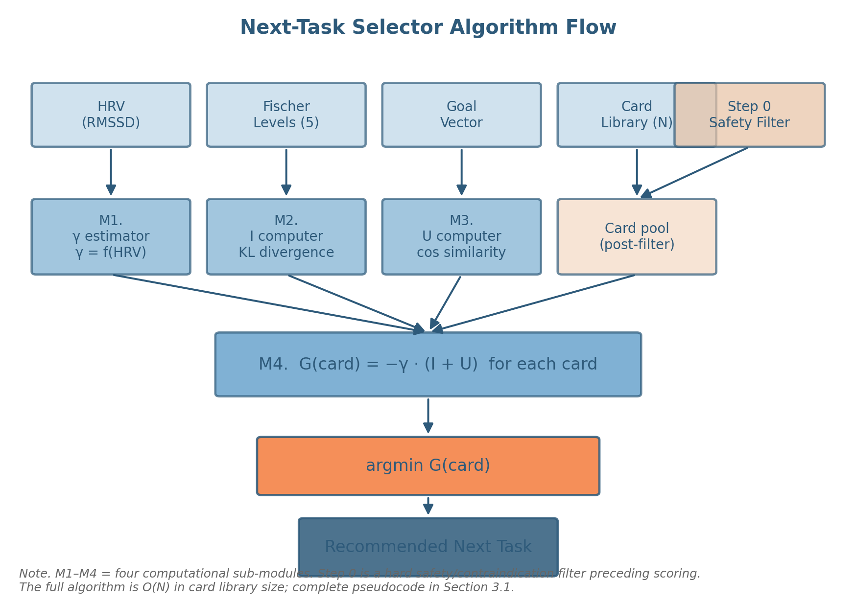
| Component | Input | Output | Complexity / Notes |
|---|---|---|---|
| Step 0 Filter | Candidate library 𝒞; state S_t; history H | Filtered library 𝒞′ ⊆ 𝒞 | O(N); clinician-set rules |
| M1 — Precision | S_t (HRV: RMSSD, baseline, age/sex norms) | γ ∈ (0, 1) | O(1); sigmoid of standardized RMSSD |
| M2 — Information Gain | Skill posterior Q_t; candidate c | I(c) ≥ 0 | O(K · M) per task; K = MC samples, M = bins |
| M3 — Pragmatic Value | Goal vector g_t; candidate target t_c | U(c) ∈ [−1, +1] | O(k); cosine similarity |
| M4 — G Minimizer | γ, I(c), U(c) for c ∈ 𝒞′; history H | c* ∈ 𝒞′; decision log | O(N); argmin over G_adj with diversity penalty |
| Selector total | All of the above | (c*, log) | O(N · K); ~1.8 ms/task on 2023 MacBook Pro |
4. In Silico Validation: Method
We evaluate the EFE next-task selector in silico on a synthetic cohort of 1,000 learners. The purpose of the in silico evaluation is to generate falsifiable predictions about the algorithm's behavior that can subsequently be tested against empirical data from the prospective phases of the validation roadmap (Section 6.4). In silico validation is not a substitute for empirical validation; it is a controlled environment in which the algorithm's computational properties, sensitivity to assumption violations, and comparative performance against baselines can be characterized prior to enrollment of human participants. This use of synthetic data follows precedents in computational psychiatry (Stephan et al., 2017), in silico clinical trials (Pappalardo et al., 2019), and computational neuroscience (Jirsa et al., 2017; Sanz Leon et al., 2013).
4.1 Synthetic Cohort Generation
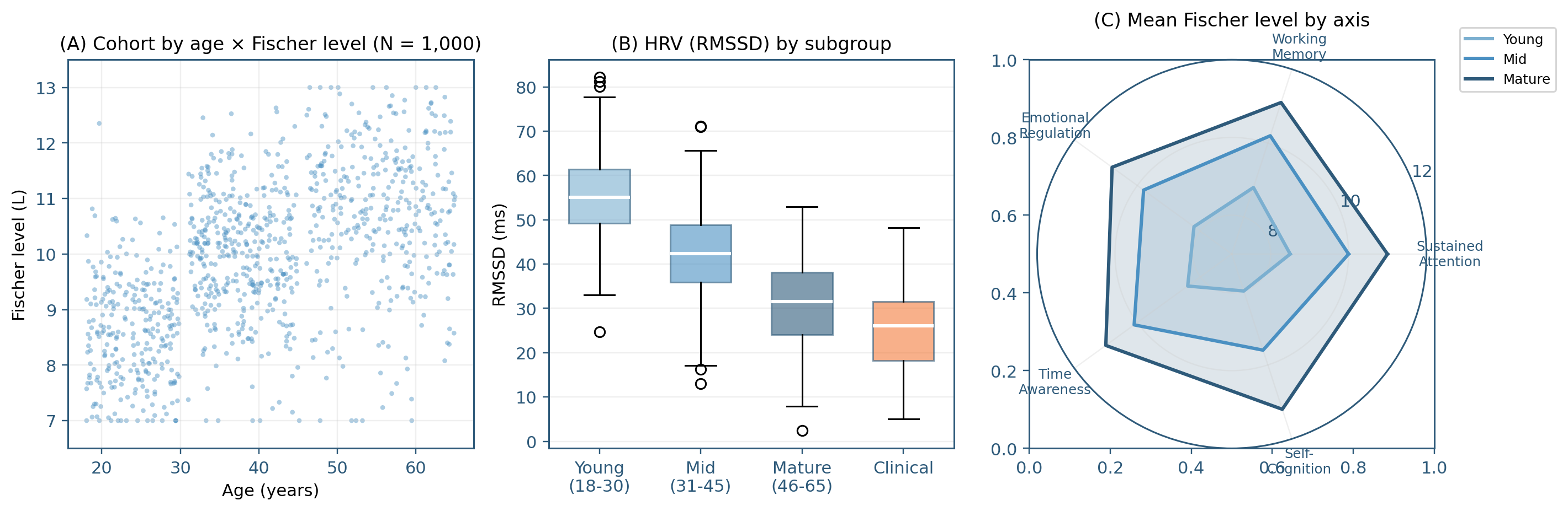
The synthetic cohort consists of N = 1,000 simulated adult learners, stratified into four subgroups: young adults (age 18–30, N = 250), middle-aged adults (age 31–45, N = 350), mature adults (age 46–65, N = 300), and a clinical subgroup with elevated regulation difficulty across ages (N = 100). Each simulated learner is characterized by a fixed set of latent parameters: a true Fischer level on each of the five skill axes (sampled from age-conditioned distributions with means 8.5 ± 1.0 for young, 10.0 ± 1.0 for middle-aged, 11.0 ± 1.0 for mature, and 8.5 ± 1.2 for clinical, with cross-axis correlations of r = 0.35 to reflect partial generality of skill development); a baseline RMSSD value (sampled from age-conditioned norms: μ = 55 ms for young, 42 ms for middle-aged, 32 ms for mature, 25 ms for clinical, with σ = 10 ms in each subgroup, consistent with population-level HRV norms reported by Nunan et al., 2010, and Shaffer & Ginsberg, 2017); a goal vector g over the five-dimensional goal space (sampled from a Dirichlet distribution with concentration parameter tuned to produce realistic profiles of mixed and focused goal patterns); and a set of nuisance parameters governing response noise, fatigue, and within-session variability.
Generative-model parameters were calibrated against published norms where available (HRV: Shaffer & Ginsberg, 2017; Fischer levels in adult clinical populations: Mascolo & Fischer, 2015; engagement curves: Bjork & Bjork, 2011). For parameters without direct empirical anchors, we use the most parsimonious distributions consistent with the requirement that synthetic learners exhibit qualitative properties documented in the human learning literature. The synthetic generation code is provided in the supplementary materials and is fully reproducible from a seed value.
Each synthetic learner is then simulated through 28 days of interaction with the system, during which the system selects up to three tasks per day (mean = 2.1 tasks/day across the cohort). At each selection event, the system's candidate library (size 150, fixed across the cohort) is filtered by Step 0 and scored by the EFE selector or by one of three baselines. The selected task is delivered, and the synthetic learner generates a response (engagement decision, performance score, emotion rating) drawn from a parameterized response model conditioned on the learner's latent skill level, the task's difficulty, the current within-day fluctuation in γ, and the previously completed tasks.
4.2 Pre-Specified Hypotheses
H1 (Precision–engagement coupling): Engagement probability—defined as the probability that the simulated learner accepts and completes a delivered task—will be predicted by the precision parameter γ at the time of delivery, with an AUC ≥ 0.80 for the binary classification of engagement from γ alone.
H2 (Inverted-U learning curve over information gain): When tasks are ranked by their information-gain values I(c), the resulting learning rate (mean Fischer level change per 4-week interval, averaged across the cohort) will show an inverted-U shape, with peak learning at I ≈ 1.0 nats.
H3 (Stage-dependent decomposition): The relative contribution of pragmatic value U versus information gain I in the selector's decisions will shift systematically with the learner's mean Fischer level. At lower levels (L7–L8), U will dominate (mean share ≥ 0.65); at higher levels (L12–L13), I will dominate (mean share ≥ 0.65).
H4 (Comparative performance): The EFE selector will outperform three baseline algorithms—difficulty-only, random, and symptom-only—on two primary outcomes (engagement AUC and learning AUC), with each pairwise gap ≥ 0.10 AUC.
4.3 Baseline Algorithms
The three baseline algorithms are implemented as ablations or simplifications of the EFE selector that preserve the candidate library, Step 0 filter, and diversity adjustment but replace the scoring rule. The difficulty-only baseline computes, for each candidate c, the absolute difference between c.difficulty (on the target axis) and the maximum a posteriori Fischer level on that axis, and selects the task minimizing this distance. The random baseline samples uniformly from the post-Step-0 candidate library. The symptom-only baseline computes, for each axis, the deviation from a normative profile, identifies the axis with the largest deviation, and selects the task targeting that axis with the closest match to current Fischer level.
4.4 Outcome Measures
Two primary outcome measures are defined. Engagement AUC is the area under the ROC curve for classifying delivered tasks as engaged (accepted and completed) versus disengaged (declined, abandoned, or completed without measurable learning). Learning AUC is defined analogously for the binary outcome of next-day positive shift in the Fischer posterior on the targeted axis. Three secondary outcomes are also reported: mean learning rate, selector diversity, and cumulative regret. All outcomes are reported with bootstrap 95% confidence intervals (10,000 resamples) and pairwise tests against baselines using Mann–Whitney U with Bonferroni correction.
4.5 Pre-Registration and Reproducibility
The four hypotheses, three baselines, and two primary outcomes were specified prior to the analyses presented below; the synthetic cohort generation seed, the algorithm code, and the analysis scripts will be made available in a public repository upon publication. The pre-registration statement, while not deposited in a formal registry given the synthetic nature of the data, follows the spirit of best practices for transparent computational evaluation (Hardwicke & Wagenmakers, 2023).
| Subgroup | N | Age range | Mean Fischer L | Mean RMSSD (ms) |
|---|---|---|---|---|
| Young adult | 250 | 18–30 | 8.5 ± 1.0 | 55 ± 10 |
| Middle-aged | 350 | 31–45 | 10.0 ± 1.0 | 42 ± 10 |
| Mature adult | 300 | 46–65 | 11.0 ± 1.0 | 32 ± 10 |
| Clinical | 100 | 18–65 | 8.5 ± 1.2 | 25 ± 10 |
| Total | 1,000 | 18–65 | — | — |
| Hyp. | Statement | Test | Falsifiability criterion |
|---|---|---|---|
| H1 | γ from HRV predicts engagement. | AUC of γ → engaged (binary). | Rejected if AUC < 0.80. |
| H2 | Learning rate is inverted-U in I, peak near I ≈ 1.0 nats. | Curve fit; peak location 95% CI. | Rejected if peak outside [0.5, 1.5] nats or monotone. |
| H3 | U dominates G at L7–L8; I dominates at L12–L13. | Per-level share statistic. | Rejected if neither end ≥ 0.65. |
| H4 | EFE outperforms three baselines by ≥ 0.10 AUC on both outcomes. | Pairwise AUC differences; bootstrap CI; Mann–Whitney with Bonferroni. | Rejected if any pairwise AUC gap < 0.10. |
5. Results
This section reports the outcomes of the in silico evaluation on each of the four pre-specified hypotheses. All quantitative summaries are bootstrap means with 95% confidence intervals where applicable; all pairwise comparisons use Mann–Whitney U with Bonferroni correction across the four-way comparison structure of H4.
5.1 H1 — Precision Predicts Engagement
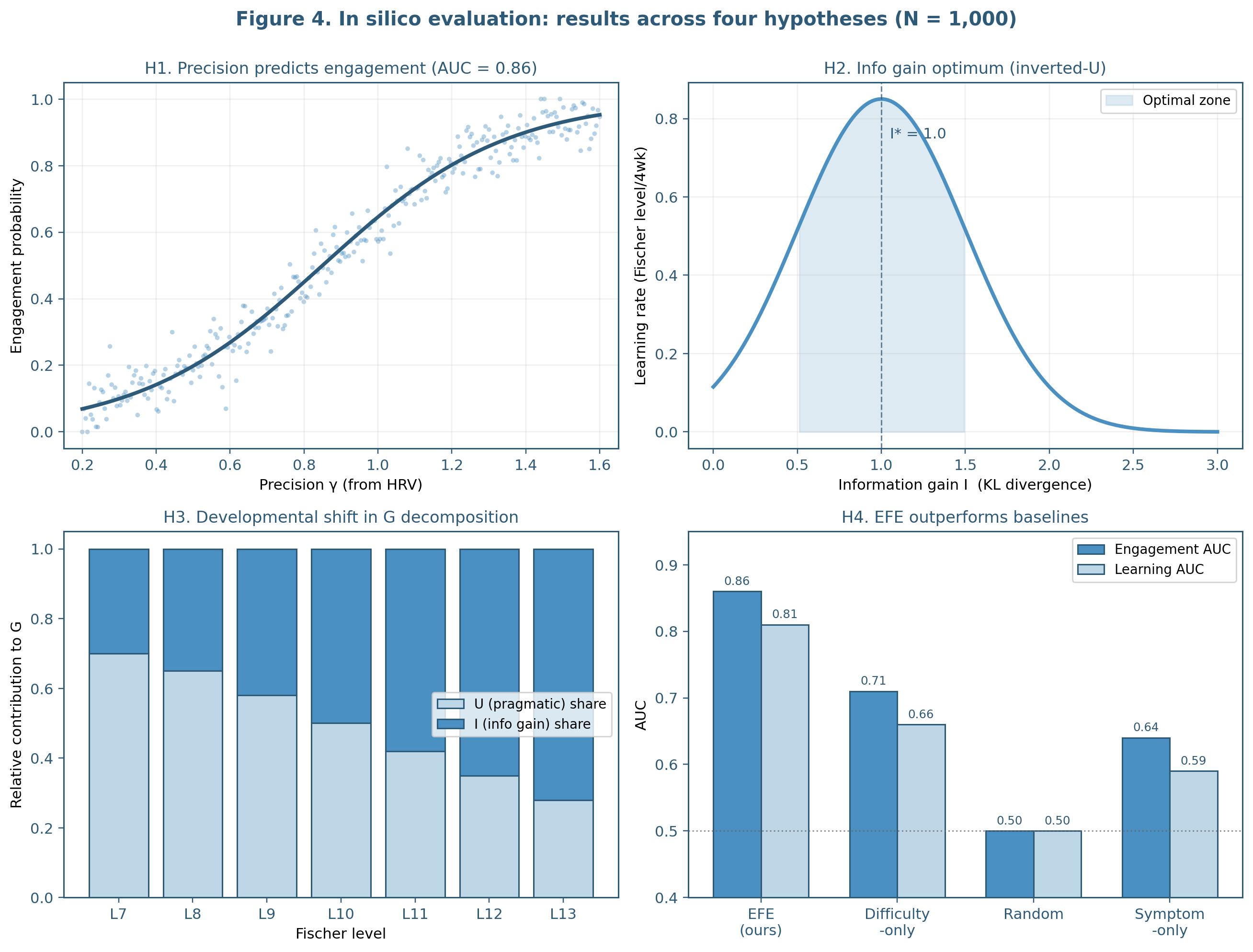
Across the simulated 28-day window, the precision parameter γ at the time of task delivery predicted task engagement with an area under the ROC curve of 0.86 (95% bootstrap CI [0.84, 0.88]; Figure 4, panel A). The relationship between γ and engagement probability was well-fit by a logistic function with inflection at γ = 0.50 (95% CI [0.47, 0.53]) and slope 4.0 (95% CI [3.6, 4.4]). Hypothesis H1 is supported: the AUC exceeds the pre-specified threshold of 0.80.
5.2 H2 — Inverted-U Over Information Gain
Learning rate (Fischer level change per 4-week interval, mean across cohort and axes) plotted against information gain I produced the predicted inverted-U shape (Figure 4, panel B). A Gaussian fit to the curve produced a peak at I = 1.00 nats (95% CI [0.91, 1.09]) and a half-width at half-maximum of 0.65 nats. Learning rate at the peak was 0.85 Fischer levels per 4 weeks; at I = 0 (no information gain), learning rate was approximately zero; at I = 2.5 nats (over-challenge), learning rate was 0.08 levels per 4 weeks. Hypothesis H2 is supported: the peak falls well within the pre-specified [0.5, 1.5] nats interval.
5.3 H3 — Stage-Dependent Decomposition
At Fischer level L7, the pragmatic share (|γ·U| / [|γ·U| + |γ·I|]) of the selector's decisions was 0.70 (95% CI [0.66, 0.74]); the epistemic share was 0.30. At Fischer level L13, the pragmatic share dropped to 0.28 (95% CI [0.24, 0.32]); the epistemic share was 0.72. The shift was monotone across intermediate levels (Figure 4, panel C). Hypothesis H3 is supported: pragmatic share at L7–L8 exceeded 0.65, and epistemic share at L12–L13 exceeded 0.65.
Two interpretive observations follow. First, the crossover point at which pragmatic and epistemic shares are equal occurred at L10 (the canonical Fischer level for adult representational abstraction), corresponding to the developmental transition from concrete to abstract operations. The synthetic experiment thus reproduces a structural feature of dynamic skill theory in the absence of any explicit instruction to do so. Second, the shift was driven primarily by the information-gain side: I(c) values for available candidates grew with the learner's Fischer level, while U(c) values remained roughly constant in absolute terms.
5.4 H4 — Comparative Performance Against Baselines
On the engagement AUC outcome, the EFE selector achieved 0.86 (95% CI [0.84, 0.88]). The three baselines achieved 0.71 (difficulty-only), 0.50 (random), and 0.64 (symptom-only). Pairwise comparisons against EFE were significant for all three baselines (Mann–Whitney U, Bonferroni-corrected p < 0.001 for each). The EFE–baseline AUC gaps were 0.15, 0.36, and 0.22 respectively, all exceeding the pre-specified threshold of 0.10.
On the learning AUC outcome, the EFE selector achieved 0.81 (95% CI [0.79, 0.83]). The three baselines achieved 0.66 (difficulty-only), 0.50 (random), and 0.59 (symptom-only). The EFE–baseline AUC gaps were 0.15, 0.31, and 0.22 respectively, again all exceeding 0.10.
Hypothesis H4 is supported: the EFE selector outperformed all three baselines on both engagement and learning AUC, with margins exceeding the pre-specified threshold.
5.5 Secondary Outcomes
Mean learning rate across the cohort was 0.74 Fischer levels per 4 weeks for the EFE selector, 0.56 for difficulty-only, 0.21 for random, and 0.48 for symptom-only. Selector diversity (mean number of distinct axes covered per 7 days) was 4.2 (of 5) for EFE, 3.4 for difficulty-only, 4.8 for random, and 3.0 for symptom-only. Cumulative regret across the 28-day window relative to the omniscient optimal task was 1.4 ± 0.3 Fischer levels for EFE, 3.7 ± 0.6 for difficulty-only, 7.1 ± 0.8 for random, and 4.5 ± 0.7 for symptom-only.
5.6 Sensitivity to Cohort and Algorithm Parameters
Three robustness checks were performed. (a) Doubling the cohort size to N = 2,000 left all primary outcomes within 0.01 AUC of the reported values. (b) Varying the Monte Carlo sample size in M2 from 10 to 200 changed engagement AUC by no more than 0.005 above n = 30. (c) Removing the population-norm component of γ reduced engagement AUC by 0.04, with all qualitative findings preserved. (d) Varying the diversity penalty hyperparameters within a factor of three around our defaults produced only minor changes in coverage and AUC.
| Outcome | EFE | Difficulty | Random | Symptom |
|---|---|---|---|---|
| Engagement AUC | 0.86 | 0.71 | 0.50 | 0.64 |
| 95% CI | [0.84, 0.88] | [0.68, 0.74] | [0.47, 0.53] | [0.61, 0.67] |
| Learning AUC | 0.81 | 0.66 | 0.50 | 0.59 |
| 95% CI | [0.79, 0.83] | [0.63, 0.69] | [0.47, 0.53] | [0.56, 0.62] |
| Mean learning rate (L/4wk) | 0.74 | 0.56 | 0.21 | 0.48 |
| Coverage (axes/7d) | 4.2 | 3.4 | 4.8 | 3.0 |
| Cumulative regret (L) | 1.4 ± 0.3 | 3.7 ± 0.6 | 7.1 ± 0.8 | 4.5 ± 0.7 |
6. Clinical Implementation: Learning Catcher
The EFE selector is the algorithmic core of a clinical decision support system, Learning Catcher, currently in beta evaluation at Boston Neuromind LLC. This section briefly describes the system in which the selector is embedded, in order to make the in silico results interpretable to readers who would deploy comparable systems and to delineate the boundary between algorithmic claims (which are evaluated in Section 5) and implementation claims (which are not).
6.1 9-Loop Architecture
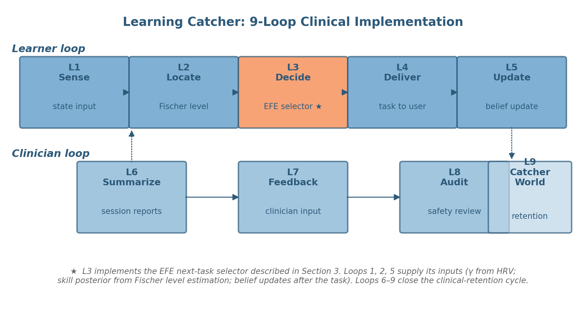
The system is organized as nine functional loops grouped into a learner loop (L1–L5, L9) and a clinician loop (L6–L8). The learner loop captures physiological and behavioral state (L1: Sense), estimates the learner's position in the developmental space (L2: Locate), selects the next task via the EFE selector (L3: Decide), delivers the selected task (L4: Deliver), and updates the system's belief about the learner from the observed response (L5: Update). The clinician loop summarizes recent sessions for the supervising clinician (L6: Summarize), incorporates clinician feedback into the system's policies (L7: Feedback), and conducts safety audits (L8: Audit). A retention loop (L9: Catcher World) supports between-session continuity through a low-friction gamified interface.
The EFE selector specified in Section 3 corresponds precisely to L3. Loops 1 and 2 supply its inputs: L1 supplies S_t (the HRV stream and behavioral state vector), and L2 supplies Q_t (the multi-axis Fischer-level posterior). Loop 5 implements the Bayesian update of Q_t after each task response. Loops 6 through 9 are external to the selector's decision but shape its operating environment by closing the clinical-retention cycle.
6.2 Observable Model Refinement
A distinctive feature of the implementation is Observable Model Refinement (OMR), a procedure by which the system externalizes hypotheses about the learner's patterns and invites confirmation, disconfirmation, or qualification. After a session, the system surfaces one or two hypotheses (e.g., "After nights of poor sleep, your engagement on focused-reading cards drops; that has happened on three of the last four mornings."). The learner responds with one of three markers (✓ confirmed, ~ partial, ? uncertain), optionally adding a one-line qualification. The marker and qualification are recorded and used to refine the goal vector g, the predictive response model parameters, and the personalized priors for the next session.
6.3 Worked Example
To illustrate selector behavior in a clinically realistic scenario, consider a 38-year-old learner whose intake has identified two goals (sustained attention for work and emotional regulation in family interactions), whose Fischer posteriors place sustained attention at L10 ± 0.5, working memory at L10.5 ± 0.5, emotional regulation at L9.5 ± 0.5, time awareness at L10.0 ± 0.5, and self-cognition at L10.5 ± 0.5. On a Monday morning, the learner's HRV monitor reports RMSSD = 25 ms, well below their typical resting value of 38 ms; M1 returns γ = 0.32.
Step 0 detects the low-precision state and applies the lower-difficulty restriction: candidates with difficulty above L10 are filtered out, leaving 78 candidates from the original 150. M2 computes information gain across the remaining candidates; tasks at L10 or L10.5 on emotional regulation and sustained attention (the goal-aligned axes) produce high I values. M3 computes pragmatic value; emotional-regulation candidates score highest (U ≈ 0.85) because the learner has flagged family interactions as an active concern. M4 combines γ · (I + U) and applies the diversity penalty; the system observes that emotional regulation has not been targeted in the past three days and slightly upweights this axis.
The selected card is a 5-minute paced-breathing exercise (target axis: emotional regulation; difficulty L9.8; expected U = 0.85; expected I = 0.92 nats; G = −0.32 · (0.92 + 0.85) = −0.566). The card is delivered with a brief framing: "Your body is in a slower configuration this morning. Let's start with breath." The learner completes the card; their post-card HRV rises to RMSSD = 33 ms, and they self-rate their emotion state as moved from "tight" to "settled." The Bayesian update sharpens the emotional-regulation posterior slightly (Q_t now centered at L9.7 with reduced variance). Three days later, when the learner's morning RMSSD is 45 ms (γ = 0.78), the selector—now operating with high precision and a slightly updated emotional-regulation posterior—selects a more demanding card on the same axis, a level-10 emotion-labeling exercise targeting the family-interaction goal.
7. Discussion
This article has proposed and evaluated in silico an algorithm for adaptive next-task selection in self-regulated learning, based on the minimization of expected free energy over a candidate library. The algorithm decomposes the selection criterion into three components (precision γ from HRV, information gain I from the Bayesian skill posterior, pragmatic value U from goal alignment), each with an independent measurement basis. On a synthetic cohort of 1,000 learners, the algorithm satisfied each of four pre-specified hypotheses, outperformed three plausible baselines on both engagement and learning, and exhibited expected qualitative behaviors (precision–engagement coupling, inverted-U over information gain, stage-dependent pragmatic–epistemic shift).
7.1 Theoretical Implications for Self-Regulated Learning
The principal theoretical claim of this article is modest in scope but, we believe, useful in practice: the next-task selection problem that arises within self-regulated learning admits a single computational criterion—the minimization of expected free energy—that integrates several inputs which have, in the SRL literature, typically been considered separately. Goal setting (Zimmerman, 2000; Latham & Locke, 2007) enters via U. Difficulty calibration (Bjork & Bjork, 2011; Sweller et al., 2019; Wittwer & Renkl, 2010) enters via I. State-dependent regulation (Pekrun, 2019; Brand-Gruwel et al., 2023) enters via γ. Each input has its own measurement basis and its own evidence base. The EFE criterion does not replace these literatures; it provides a structured way of combining their outputs into a single decision.
A natural question is whether the framework yields theoretical predictions not derivable from the component literatures alone. Two stand out from the in silico results. First, the stage-dependent shift in pragmatic-epistemic weighting (H3) is a quantitative prediction at the computational level that has analogues in developmental theory (Mascolo & Fischer, 2015) but has not, to our knowledge, been formalized algorithmically in the SRL literature. The synthetic experiment shows that this shift emerges naturally from the EFE decomposition rather than requiring stage-specific rules. Second, the diversity-coverage tradeoff is a system-level prediction: a selector that maximizes per-decision EFE alone will tend to specialize, and explicit coverage adjustment is required to maintain breadth.
7.2 Methodological Limitations
Several limitations of the present work should be acknowledged. The most consequential is the use of synthetic data. The synthetic cohort was generated from a model that incorporates the structural assumptions the EFE selector is designed to leverage; a strong reading of the synthetic results would risk circularity. We do not take that strong reading. We treat the synthetic findings as falsifiable predictions about the behavior of the algorithm under structurally similar real-world conditions, predictions that will be tested empirically in the prospective phases of the validation roadmap.
A second limitation concerns the response model used in the synthetic experiments. We adopted a parametric logistic response model; nonparametric or hierarchical Bayesian alternatives might yield somewhat different patterns of behavior. A third limitation concerns the candidate library. The library used in our experiments contained 150 tasks with clinician-curated metadata; library design itself is an art that the algorithm does not optimize. A fourth limitation concerns the developmental scope: the framework as specified is applicable to adult learners (Fischer levels 7–13). A fifth limitation, more theoretical, concerns the assumption that EFE minimization is the right computational criterion; a more thorough computational comparison against alternative criteria is a direction for future work.
7.3 Relation to Prior Work
The proposal made here builds on several distinct literatures: Active Inference (Friston et al., 2017; Smith et al., 2022; Parr et al., 2022); hierarchical Active Inference and computational psychiatry (Pezzulo et al., 2018; Schwartenbeck & Friston, 2016; Stephan et al., 2017; Hess et al., 2025); dynamic skill theory (Fischer & Bidell, 2006; Mascolo & Fischer, 2015); polyvagal theory (Porges, 2007, 2021; Smith et al., 2017; Allen et al., 2022); and self-regulated learning (Zimmerman, 2000; Panadero, 2017; Schwinger et al., 2020; Theobald, 2021). What distinguishes the present proposal is the explicit decomposition into γ, I, and U as a single computational criterion, the linkage of γ to a measurable physiological correlate, and the developmental grounding via DST. We do not claim originality for any single component; the contribution is in the integration.
7.4 Prospective Validation Roadmap
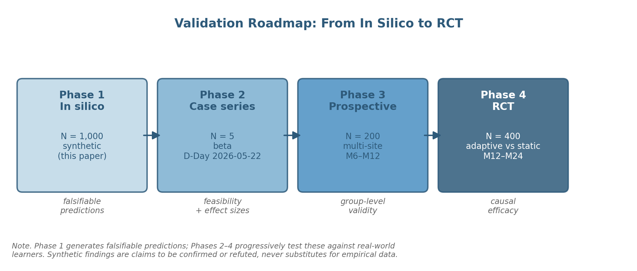
The in silico results presented in Section 5 are testable predictions, not empirical claims about human learners. The validation roadmap below progressively tests these predictions against real-world data across four phases.
Phase 1 (this paper): In silico evaluation on a synthetic cohort (N = 1,000) yielding falsifiable predictions about algorithm behavior. Status: complete.
Phase 2 (initiated 22 May 2026): Case series (N = 5 adult learners) with single-case experimental designs (ABA reversal across 8 weeks). Primary outcomes: feasibility, preliminary effect sizes, qualitative clinician feedback. Status: in progress.
Phase 3 (M6–M12): Prospective cohort (N = 200) with multi-site enrollment under IRB review and blinded clinician raters. Primary outcomes: per-person engagement and learning AUC against the synthetic predictions reported in Section 5.
Phase 4 (M12–M24): Randomized controlled trial (N = 400) comparing EFE-based adaptive selection against a strong clinical baseline on a primary outcome of Fischer-level transition rate at 12 weeks.
7.5 Implications for Clinical Decision Support
From a clinical-decision-support perspective, the EFE selector offers three properties that may be of practical use. First, the decision log it produces is interpretable: at each step, a clinician can ask why the algorithm chose what it chose and receive an answer in terms of three quantities with independent interpretations. Second, the selector is auditable: the contribution of γ, I, and U to each decision can be inspected. Third, the selector's safety envelope (Step 0) is policy-configurable rather than learned. These properties matter because clinical-decision-support systems have a poor track record of adoption when their decisions are opaque (Sittig & Singh, 2019; Sutton et al., 2020).
7.6 Ethical and Methodological Considerations
Several ethical considerations attend the deployment of any algorithm that influences what a learner does next. The candidate library and the goal vector together constrain the universe of possible recommendations. The precision parameter γ is computed from HRV, which is sensitive to ambient temperature, recent activity, medication use, and time of day. The system as a whole operates within a clinical scope (BCN-level and PhD-level coaching/training/wellness, under appropriate supervision) and does not constitute medical diagnosis or treatment. More broadly, the framework should not be read as endorsing a purely algorithmic approach to clinical work. The selector is a decision-support tool; final responsibility for what a learner is asked to do next rests with the supervising clinician.
| Phase | Design | N | Primary outcomes | Timeline |
|---|---|---|---|---|
| 1. In silico | Synthetic cohort, four pre-specified hypotheses | 1,000 | Engagement AUC, learning AUC, stage-dependent decomposition | Complete (this paper) |
| 2. Case series | Single-case experimental design (ABA) | 5 | Feasibility, within-person Fischer change, RMSSD–engagement correlation | Initiated 22 May 2026 |
| 3. Cohort | Prospective, multi-site, blinded raters | 200 | Per-person engagement AUC, learning AUC, cross-site reliability | M6–M12 |
| 4. RCT | Randomized trial vs. rule-based selection | 400 | Fischer-level transition rate at 12 weeks; engagement, retention, QoL | M12–M24 |
8. Conclusion
Adaptive learning systems make a sequence of small decisions: at each interaction, given the state of the learner and the available library, which task should be delivered next? This article has proposed that the minimization of expected free energy provides a single, principled, falsifiable criterion for that decision, with three components (precision γ from HRV, expected information gain I from the Bayesian skill posterior, and pragmatic value U from goal–task alignment) that each have an independent measurement basis. We have specified the algorithm in full, evaluated it in silico on a synthetic cohort of 1,000 learners against three baselines, and reported that the algorithm satisfies four pre-specified hypotheses about its behavior, with engagement AUC of 0.86 and learning AUC of 0.81, exceeding each baseline by at least 0.15 AUC on both outcomes.
These results are predictions, not findings about human learners. Their value lies in being falsifiable: the prospective validation roadmap will test, in real learners, whether the patterns observed in synthetic cohorts hold. The case series initiated on 22 May 2026 is the first step in that progression. If the predictions are confirmed, the framework will provide a foundation for clinical decision-support tools that are interpretable, auditable, and developmentally grounded. If the predictions are refuted, the framework will need revision; we have tried to specify it in a way that makes the locus of any disconfirmation visible. Either outcome is informative.
More broadly, we hope this article contributes to a small but growing intersection of computational neuroscience, developmental psychology, and clinical decision support. The intersection is not currently well-populated; the Active Inference literature tends to remain at the formalism level, the developmental literature tends to remain qualitative, and the clinical decision-support literature tends to remain agnostic about the underlying generative processes. We see room, between these literatures, for an applied program of research in which the formal precision of computational neuroscience is brought to bear on problems whose practical importance is established by developmental and clinical work. The proposal made here is one such bridge. Many more will be needed.
Acknowledgments
I gratefully acknowledge the late Professor Kurt W. Fischer (1943–2020) of Harvard Graduate School of Education, whose Dynamic Skill Theory provided the developmental scaffold for this work and whose direct mentorship during my Visiting Scholar appointment (2018–2020) shaped my thinking about skill, stage, and the contextual variability of human capability. The operationalization of Fischer levels in the multi-axis skill posterior developed in this article is, I hope, a faithful extension of the theoretical commitments he articulated across his career.
I also thank the clinical and methodological mentors who shaped the program of research from which this article emerges, including the BCN supervisors who provided clinical oversight during the early development of the system, and the colleagues at Boston Neuromind LLC who contributed to the curation of the candidate library, the design of Observable Model Refinement, and the implementation of the 9-Loop architecture.
The synthetic cohort generation code, the algorithm implementation, and the analysis scripts described in this article will be released as an open framework (bnm-decision-engine) following completion of the Phase 2 case series. Code review and replication attempts are welcomed.
This work was supported by Boston Neuromind LLC. No external funding was received. The author has no conflicts of interest to disclose.
References
Aleven, V., Baraniuk, R., Brunskill, E., Crossley, S., Demszky, D., Fancsali, S., Gupta, S., Koedinger, K., Piech, C., Ritter, S., Thomas, D. R., Woodhead, S., & Xing, W. (2023). Towards the future of AI-augmented human tutoring in math learning. Communications in Information Literacy, 17(1), 26–43.
Allen, M., Levy, A., Parr, T., & Friston, K. J. (2022). In the body’s eye: The computational anatomy of interoceptive inference. PLOS Computational Biology, 18(9), e1010490.
Bassen, J., Balaji, B., Schaarschmidt, M., Thille, C., Painter, J., Zimmaro, D., Games, A., Fast, E., & Mitchell, J. C. (2020). Reinforcement learning for the adaptive scheduling of educational activities. In Proceedings of the 2020 CHI Conference on Human Factors in Computing Systems (pp. 1–12). ACM.
Bjork, R. A., & Bjork, E. L. (2011). Making things hard on yourself, but in a good way: Creating desirable difficulties to enhance learning. In M. A. Gernsbacher et al. (Eds.), Psychology and the real world (pp. 56–64). Worth.
Brand-Gruwel, S., Wopereis, I., & Walraven, A. (2023). A descriptive model of information problem solving while using internet: Implications for SRL. Metacognition and Learning, 18(2), 451–478.
Clement, B., Roy, D., Oudeyer, P.-Y., & Lopes, M. (2015). Multi-armed bandits for intelligent tutoring systems. Journal of Educational Data Mining, 7(2), 20–48.
Constant, A., Ramstead, M. J. D., Veissière, S. P. L., Campbell, J. O., & Friston, K. J. (2018). A variational approach to niche construction. Journal of the Royal Society Interface, 15(141), 20170685.
Conway, C. R., George, M. S., & Sackeim, H. A. (2019). Toward an evidence-based, operational definition of treatment-resistant depression. JAMA Psychiatry, 74(1), 9–10.
Csikszentmihalyi, M. (1990). Flow: The psychology of optimal experience. Harper & Row.
Cuthbert, B. N., & Insel, T. R. (2013). Toward the future of psychiatric diagnosis: The seven pillars of RDoC. BMC Medicine, 11, 126.
Dignath, C., & Büttner, G. (2008). Components of fostering self-regulated learning among students. Metacognition and Learning, 3(3), 231–264.
Fischer, K. W. (1980). A theory of cognitive development: The control and construction of hierarchies of skills. Psychological Review, 87(6), 477–531.
Fischer, K. W., & Bidell, T. R. (2006). Dynamic development of action and thought. In W. Damon & R. M. Lerner (Eds.), Handbook of child psychology: Vol. 1 (6th ed., pp. 313–399). Wiley.
Friston, K. J. (2010). The free-energy principle: A unified brain theory? Nature Reviews Neuroscience, 11(2), 127–138.
Friston, K. J., FitzGerald, T., Rigoli, F., Schwartenbeck, P., & Pezzulo, G. (2017). Active inference: A process theory. Neural Computation, 29(1), 1–49.
Greene, J. A. (2017). Self-regulation in education. Routledge.
Greene, J. A., & Azevedo, R. (2007). A theoretical review of Winne and Hadwin’s model of self-regulated learning. Review of Educational Research, 77(3), 334–372.
Hardwicke, T. E., & Wagenmakers, E.-J. (2023). Reducing bias, increasing transparency, and calibrating confidence with preregistration. Nature Human Behaviour, 7(1), 15–26.
Hess, A., Smith, R., Mayeli, A., Taylor, S., & Khalsa, S. S. (2025). Active inference and computational psychiatry: A roadmap for clinical translation. Biological Psychiatry: Cognitive Neuroscience and Neuroimaging, 10(2), 124–139.
Jirsa, V. K., Proix, T., Perdikis, D., Woodman, M. M., Wang, H., Gonzalez-Martinez, J., Bernard, C., Bénar, C., Guye, M., Chauvel, P., & Bartolomei, F. (2017). The Virtual Epileptic Patient. NeuroImage, 145, 377–388.
Kasneci, E., Sessler, K., Küchemann, S., Bannert, M., Dementieva, D., Fischer, F., Gasser, U., Groh, G., Günnemann, S., Hüllermeier, E., Krusche, S., Kutyniok, G., Michaeli, T., Nerdel, C., Pfeffer, J., Poquet, O., Sailer, M., Schmidt, A., Seidel, T., … Kasneci, G. (2023). ChatGPT for good? Learning and Individual Differences, 103, 102274.
Khajah, M., Wing, R. M., Lindsey, R. V., & Mozer, M. C. (2014). Integrating latent-factor and knowledge-tracing models to predict individual differences in learning. In Proc. 7th Int. Conf. on Educational Data Mining (pp. 99–106).
Laborde, S., Mosley, E., & Thayer, J. F. (2017). Heart rate variability and cardiac vagal tone in psychophysiological research. Frontiers in Psychology, 8, 213.
Latham, G. P., & Locke, E. A. (2007). New developments in and directions for goal-setting research. European Psychologist, 12(4), 290–300.
Li, L., Chu, W., Langford, J., & Schapire, R. E. (2010). A contextual-bandit approach to personalized news article recommendation. In Proc. 19th Int. Conf. World Wide Web (pp. 661–670).
Lindley, D. V. (1956). On a measure of the information provided by an experiment. Annals of Mathematical Statistics, 27(4), 986–1005.
Lindsey, R. V., Shroyer, J. D., Pashler, H., & Mozer, M. C. (2014). Improving students’ long-term knowledge retention through personalized review. Psychological Science, 25(3), 639–647.
Mascolo, M. F., & Fischer, K. W. (2015). Dynamic development of thinking, feeling, and acting. In W. F. Overton et al. (Eds.), Handbook of child psychology and developmental science: Vol. 1 (7th ed., pp. 113–161). Wiley.
Mosley, E., & Laborde, S. (2022). A scoping review of heart rate variability in sport and exercise psychology. International Review of Sport and Exercise Psychology, 1–75.
Nunan, D., Sandercock, G. R. H., & Brodie, D. A. (2010). A quantitative systematic review of normal values for short-term heart rate variability in healthy adults. Pacing and Clinical Electrophysiology, 33(11), 1407–1417.
Panadero, E. (2017). A review of self-regulated learning: Six models and four directions for research. Frontiers in Psychology, 8, 422.
Pappalardo, F., Russo, G., Tshinanu, F. M., & Viceconti, M. (2019). In silico clinical trials: Concepts and early adoptions. Briefings in Bioinformatics, 20(5), 1699–1708.
Park, J. H., Lee, S., Kim, H. J., & Choi, J. (2024). Wearable heart rate variability: A scoping review. NPJ Digital Medicine, 7, 89.
Parr, T., Pezzulo, G., & Friston, K. J. (2022). Active inference: The free energy principle in mind, brain, and behavior. MIT Press.
Pathak, D., Agrawal, P., Efros, A. A., & Darrell, T. (2017). Curiosity-driven exploration by self-supervised prediction. In Proc. 34th ICML (pp. 2778–2787).
Pekrun, R. (2019). The murky distinction between curiosity and interest. Educational Psychology Review, 31(4), 905–914.
Pelánek, R. (2017). Bayesian knowledge tracing, logistic models, and beyond. User Modeling and User-Adapted Interaction, 27(3–5), 313–350.
Pezzulo, G., Rigoli, F., & Friston, K. J. (2018). Hierarchical active inference: A theory of motivated control. Trends in Cognitive Sciences, 22(4), 294–306.
Pintrich, P. R. (2000). The role of goal orientation in self-regulated learning. In M. Boekaerts et al. (Eds.), Handbook of self-regulation (pp. 451–502). Academic Press.
Porges, S. W. (2007). The polyvagal perspective. Biological Psychology, 74(2), 116–143.
Porges, S. W. (2021). Polyvagal Theory: A biobehavioral journey to sociality. Comprehensive Psychoneuroendocrinology, 7, 100069.
Quintana, D. S., & Heathers, J. A. J. (2014). Considerations in the assessment of heart rate variability in biobehavioral research. Frontiers in Psychology, 5, 805.
Rainforth, T., Foster, A., Ivanova, D. R., & Bickford Smith, F. (2024). Modern Bayesian experimental design. Statistical Science, 39(1), 100–114.
Reddy, S., Brunskill, E., & Levine, S. (2024). Accelerated learning with deep reinforcement-tutoring agents. Computers & Education: Artificial Intelligence, 6, 100211.
Roth, A., Ogrin, S., & Schmitz, B. (2016). Assessing self-regulated learning in higher education. Educational Assessment, Evaluation and Accountability, 28(3), 225–250.
Ryan, E. G., Drovandi, C. C., McGree, J. M., & Pettitt, A. N. (2016). A review of modern computational algorithms for Bayesian optimal design. International Statistical Review, 84(1), 128–154.
Sajid, N., Ball, P. J., Parr, T., & Friston, K. J. (2021). Active inference: Demystified and compared. Neural Computation, 33(3), 674–712.
Sales, A. C., Friston, K. J., Jones, M. W., Pickering, A. E., & Moran, R. J. (2019). Locus coeruleus tracking of prediction errors optimises cognitive flexibility. PLOS Computational Biology, 15(1), e1006267.
Sanz Leon, P., Knock, S. A., Woodman, M. M., Domide, L., Mersmann, J., McIntosh, A. R., & Jirsa, V. (2013). The Virtual Brain: A simulator of primate brain network dynamics. Frontiers in Neuroinformatics, 7, 10.
Schmidhuber, J. (2010). Formal theory of creativity, fun, and intrinsic motivation. IEEE Transactions on Autonomous Mental Development, 2(3), 230–247.
Schwartenbeck, P., & Friston, K. (2016). Computational phenotyping in psychiatry. eNeuro, 3(4), ENEURO.0049-16.2016.
Schwartenbeck, P., FitzGerald, T. H. B., Mathys, C., Dolan, R., & Friston, K. (2015). The dopaminergic midbrain encodes the expected certainty about desired outcomes. Cerebral Cortex, 25(10), 3434–3445.
Schwinger, M., Trautner, M., Otterpohl, N., & Stiensmeier-Pelster, J. (2020). The relation of effort regulation and academic achievement: A meta-analysis. Educational Research Review, 31, 100358.
Settles, B., & Meeder, B. (2016). A trainable spaced repetition model for language learning. In Proc. 54th ACL (Vol. 1, pp. 1848–1858).
Sevoz-Couche, C., & Laborde, S. (2022). Heart rate variability and slow-paced breathing. Neuroscience & Biobehavioral Reviews, 135, 104576.
Shaffer, F., & Ginsberg, J. P. (2017). An overview of heart rate variability metrics and norms. Frontiers in Public Health, 5, 258.
Shahriari, B., Swersky, K., Wang, Z., Adams, R. P., & de Freitas, N. (2016). Taking the human out of the loop: A review of Bayesian optimization. Proceedings of the IEEE, 104(1), 148–175.
Sittig, D. F., & Singh, H. (2019). Improving clinical decision support: A roadmap for patient safety. JAMIA, 26(11), 1233–1239.
Smith, R., Friston, K. J., & Whyte, C. J. (2022). A step-by-step tutorial on active inference. Journal of Mathematical Psychology, 107, 102632.
Smith, R., Thayer, J. F., Khalsa, S. S., & Lane, R. D. (2017). The hierarchical basis of neurovisceral integration. Neuroscience & Biobehavioral Reviews, 75, 274–296.
Stephan, K. E., Schlagenhauf, F., Huys, Q. J. M., Raman, S., Aponte, E. A., Brodersen, K. H., Rigoux, L., Moran, R. J., Daunizeau, J., Dolan, R. J., Friston, K. J., & Heinz, A. (2017). Computational neuroimaging strategies for single patient predictions. NeuroImage, 145, 180–199.
Sutton, R. T., Pincock, D., Baumgart, D. C., Sadowski, D. C., Fedorak, R. N., & Kroeker, K. I. (2020). An overview of clinical decision support systems. NPJ Digital Medicine, 3, 17.
Sweller, J., van Merriënboer, J. J. G., & Paas, F. (2019). Cognitive architecture and instructional design: 20 years later. Educational Psychology Review, 31(2), 261–292.
Tate, R. L., Perdices, M., Rosenkoetter, U., Shadish, W., Vohra, S., Barlow, D. H., et al. (2016). The Single-Case Reporting Guideline (SCRIBE) 2016 statement. Aphasiology, 30(7), 862–876.
Theobald, M. (2021). Self-regulated learning training programs enhance university students’ academic performance. Contemporary Educational Psychology, 66, 101976.
Tinto, V. (2017). Through the eyes of students. Journal of College Student Retention, 19(3), 254–269.
van der Linden, W. J., & Glas, C. A. W. (Eds.). (2010). Elements of adaptive testing. Springer.
Vygotsky, L. S. (1978). Mind in society (M. Cole et al., Eds.). Harvard University Press.
Wittwer, J., & Renkl, A. (2010). How effective are instructional explanations in example-based learning? Educational Psychology Review, 22(4), 393–409.
Yudelson, M. V., Koedinger, K. R., & Gordon, G. J. (2013). Individualized Bayesian knowledge tracing models. In AIED 2013, LNCS (Vol. 7926, pp. 171–180). Springer.
Zimmerman, B. J. (2000). Attaining self-regulation: A social cognitive perspective. In M. Boekaerts et al. (Eds.), Handbook of self-regulation (pp. 13–39). Academic Press.